Example 1.11 A class consisting of 4 graduate and 12 undergraduate students is randomly divided into 4 groups of 4. What is the probability that each group includes a graduate student? We interpret randomly to mean that given the assignment of some students to certain slots, any of the remaining students are equally likely to be assigned to any of the remaining slots.
Solution
In the beginning, we have 16 different slots, where each group takes up 4 slots. Let G be the event that every group has one grad student.
\begin{align}
A_0 = \text{\{Grad student 1 is in different groups, but $P(A_0)=1$\}} \nonumber \\
A_1 = \text{\{Grad student 1 and 2 are in different groups\}} \nonumber \\
A_2 = \text{\{Grad student 1, 2 and 3 are in different groups\}} \nonumber \\
A_3 = \text{\{Grad student 1, 2, 3, 4 are in different groups\}} \nonumber
\end{align}
After grad student 1 has been picked only 15 people will be left, and since the available slots left are 3 we have 12 possible locations (3*4=12). Thus:
Let us see if this is really the case with a simulation
Code
import numpy as npimport randomfrom tqdm import tqdmvalid_array = []num_sim =1000# NOTE: remember to set high for better resultsfor _ inrange(num_sim): student_id = np.arange(1, 17) random.shuffle(student_id) groups = [ student_id[0:4], student_id[4:8], student_id[8:12], student_id[12:16], ] for g in groups: num_grad_in_g =0for g_id in [1,2,3,4]:if g_id in g: num_grad_in_g +=1if num_grad_in_g >1:breakif num_grad_in_g >1: valid_array.append(0)else: valid_array.append(1)print(f'Probability is {np.sum(valid_array)/float(num_sim)} after {num_sim} trials.')
Probability is 0.13 after 1000 trials.
Example 1.14. Alice is taking a probability class and at the end of each week she can be either up-to-date or she may have fallen behind. If she is up-to-date in a given week, the probability that she will be up-to-date (or behind) in the next week is 0.8 (or 0.2, respectively). If she is behind in a given week, the probability that she will be up-to-date (or behind) in the next week is 0.6 (or 0.4, respectively). Alice is (by default) up-to-date when she starts the class. What is the probability that she is up-to-date after three weeks?
Solution
Let U_i be the event that Alice is up-to-date at the end of week i and \overline{U}_i be not up-to-date, the goal is the find P(U_3).
Starting with P(U_2)=P(U_2\cap U_1)\bigcup P(U_2\cap\overline{U}_1) which becomes P(U_2) = P(U_1)P(U_2|U_1)+ P(\overline{U}_1)P(U_2|\overline{U}_1). Since she starts the week up-to-date, then P(U_1)=0.8, P(\overline{U}_1) = 0.2.
Example 1.17. Consider an experiment involving two successive rolls of a 4-sided die in which all 16 possible outcomes are equally likely and have a probability of 1/16.
Are the events A = \text{\{maximum of the two rolls is 2\}}, B = \text{\{minimum of the two rolls is 2}\} independent?
Solution
They are not independent because P(A) = 3/16, P(B) = 5/16, P(A\cap B) = 1/16 \neq 15/(16*16).
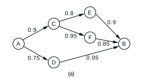
Example 1.22. Network connectivity. A computer network connects two nodes A and B through intermediate nodes C, D, E, and F. For every pair of directly connected nodes, say i and j, there is a given probability p_{ij} that the link from i to j is up. We assume that link failures are independent of each other. What is the probability that there is a path connecting A and B in which all links are up?
Solution
\begin{align}
P(l_1:= A\rightarrow D \rightarrow B) = 0.75 * 0.95 =0.7125\\
P(l_2:=C\rightarrow E \rightarrow B) = 0.8 * 0.9 =0.72\\
P(l_3:=C\rightarrow F \rightarrow B) = 0.95 * 0.85=0.8075 \\
\end{align}
The probability that l_4: C\rightarrow B has at least one successful path is :
Example 2.8. Average Speed Versus Average Time. If the weather is good (which happens with probability 0.6), Alice walks the 2 miles to class at a speed of V = 5 miles per hour, and otherwise drives her motorcycle at a speed of V = 30 miles per hour. What is the mean of the time T to get to class?
But using E[V] to find E[T] using E[T] = E[1/V] =1/E[V] doesn’t work. Because 1/x is not linear.
Example 2.11. Professor May B. Right often has her facts wrong, and answers each of her students’ questions incorrectly with probability 1/4, independently of other questions. In each lecture, May is asked 0, 1, or 2 questions with an equal probability of 1/3. Let X and Y be the number of questions May is asked and the number of questions she answers wrong in a given lecture, respectively. Construct the joint PMF p_{X,Y} (x, y)
Solution
The PMF p_{X,Y} (x, y) - defined as p_{X,Y} (x, y) = P(X=x, Y=y) - can be found by using the multiplication rule; p_{X,Y}(x,y) = p_X(x)p_{Y|X}(y|x):
y=2
0
0
1/48
y=1
0
1/12
6/48
y=0
1/3
3/12
9/48
x=0
x=1
x=2
Example 2.12. Consider four independent rolls of a 6-sided die. Let X be the number of 1’s and let Y be the number of 2’s obtained. What is the joint PMF of X and Y ?
Y is the number 2’s, so conditioned on x (the number of 1’s), the possible choices are limited to 2,3,4,5,6, and the number of 2’s required becomes 4-x
p_{Y|X}(y|x) = \dbinom{4-x}{y} \left( \frac{1}{5} \right) ^y \left( \frac{4}{5}\right) ^ {4-x-y}
Example 2.13. Consider a transmitter that is sending messages over a computer network.
Example
Let us have two random variables:
X = \text{the travel time of the message}, Y=\text{the length of the message}
We are given:
The length of a message can take two possible values: y = 10^2 bytes with probability 5/6, and y = 10^4 bytes with probability 1/6. This is the PMF of X - p_X(x).
We know that the travel time of the message depends on the length, i.e. p_{X|Y}(x|y). In particular, travel time is 10^{−4}Y secs with probability 1/2, 10^{−3}Y secs with probability 1/3, and 10^{−2}Y secs with probability 1/6.
For instance, to find the probability of the travel time of the message being 1 sec,
p_X(x=1) = 1/6 * 5*6 + 1/2*1/6
Very cool!
Example 2.15.Mean and Variance of the Geometric Random Variable.
You write a software program over and over, and each time there is a probability p that it works correctly, independently from previous attempts. What is the mean and variance of X, the number of tries until the program works correctly?
Solution
X is a geometric random variable with PMF:
p_X(k) = (1-p)^{k-1} p \quad k = 1,2,3,\dots
The mean is
E[X] = \sum_{k=1}^{\infty} k (1-p)^{k-1} p
The variance is var(X) = E((X-E(X))^2) = \sum_{k=1}^{\infty} (k - E(X))(1-p)^{k-1} p.
Let’s define P(A_1 = \{X=1\}) and P(A_2 = \{X>1\}) - meaning the first time works and the first time didn’t work, respectively.
The conditional expectation of A_1:
\begin{align}
E[X| A_1 = \{X=1\}] &= 1
\end{align}
The conditional expectation of A_2:
\begin{align}
E[X| A_2 = \{X>1\}] &= 1 + E[X]
\end{align}
This is because the first try was a failure. Thus, using the Total Expectation Theorem - E[X] = \sum_y p_Y(y) E[X|Y=y] - we have:
Example 3.5. The time until a small meteorite first lands anywhere in the Sahara desert is modeled as an exponential random variable with a mean of 10 days. The time is currently midnight. What is the probability that a meteorite first lands some time between 6am and 6pm of the first day? And, on any day?
Solution
The exponential random variable has the PDF of the form:
f_X(x) =
\begin{cases}
\lambda e ^{-\lambda x} &\quad \text{if x > 0} \\
0 &\quad \text{else}
\end{cases}
Since the mean is E[X] = 1/\lambda, then \lambda = 1/10. The unit is in days, so 6 am to 6 pm is 1/4 and 3/4, respectively.
P(1/4 < X < 3/4 ) = \int_{1/4}^{3/4} \lambda e ^{-\lambda x} dx
For any day, we need to sum all of the probabilities for each day.
P(\text{6am-6pm}) = \sum_{k=1}^{\infty} P(k - 3/4 < X < k-1/4)
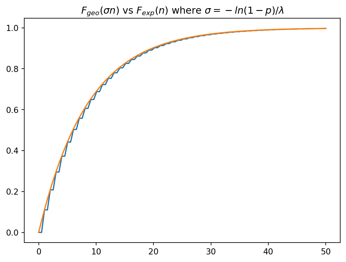
Example 3.6. The Geometric and Exponential CDFs.
Comparing geometric and exponential CDF
The CDF is defined as F(x) = P(X\leq x) \quad \forall x
F^{geo}(n) = \sum_{k=1}^{n}p(1-p) ^{k-1}
Using r = (1-p), the geometric sum is then
F^{geo}(n) = p \frac{1-(1-p)^n}{1-(1-p)} = 1-(1-p)^n
For exponential,
\begin{align}
F^{exp}(x) &= \int_{-\infty}^{x} \lambda e^{-\lambda z} dz \\
&=1 - e ^{-\lambda x} \quad \forall x >0
\end{align}
Code
import numpy as npimport matplotlib.pyplot as pltn = np.linspace(0., 50., 100)F_geo =lambda p, n: 1- np.power((1-p),np.floor(n))F_exp =lambda l, x: 1- np.exp(-l* x)p =0.11l =1/pf_geo = F_geo(p, n)sigma =-np.log(1- p)/lf_lambda = F_exp(l, n*sigma)plt.plot(n, f_geo, n, f_lambda)_ = plt.title('$F_{geo}(\sigma n)$ vs $F_{exp}(n)$ where $\sigma = -ln(1-p)/\lambda$')
Cool simulations
Monte Hall simulation
Code
import numpy as npimport randomfrom tqdm import tqdmdef mt(switch): win_array = []for _ inrange(num_sim):# 1 - car prizes = np.arange(1, 4) random.shuffle(prizes) pick_id = np.random.randint(0, 3) car_id, = np.where(prizes ==1) allowed = [0,1,2] allowed.remove(pick_id) host_allowed = allowed.copy()if prizes[pick_id] !=1: host_allowed.remove(car_id[0]) allowed.remove(host_allowed[0])if switch:if prizes[allowed[0]] ==1: win_array.append(1) else: win_array.append(0)else:if prizes[pick_id] ==1: win_array.append(1) else: win_array.append(0)return np.sum(win_array)/float(num_sim)print(f'After {num_sim} games')print(f'Probability of winning the car with switching is {mt(1)} ')print(f'Probability of winning the car without switching is {mt(0)} ')
After 1000 games
Probability of winning the car with switching is 0.66
Probability of winning the car without switching is 0.342